Chapter 2 Mask-RCNN model implementation
After our file with the list of URLs has been uploaded to Dropbox, we next implement a Region-based Convolutional Neural Network (R-CNN).
2.1 Mask R-CNN theory
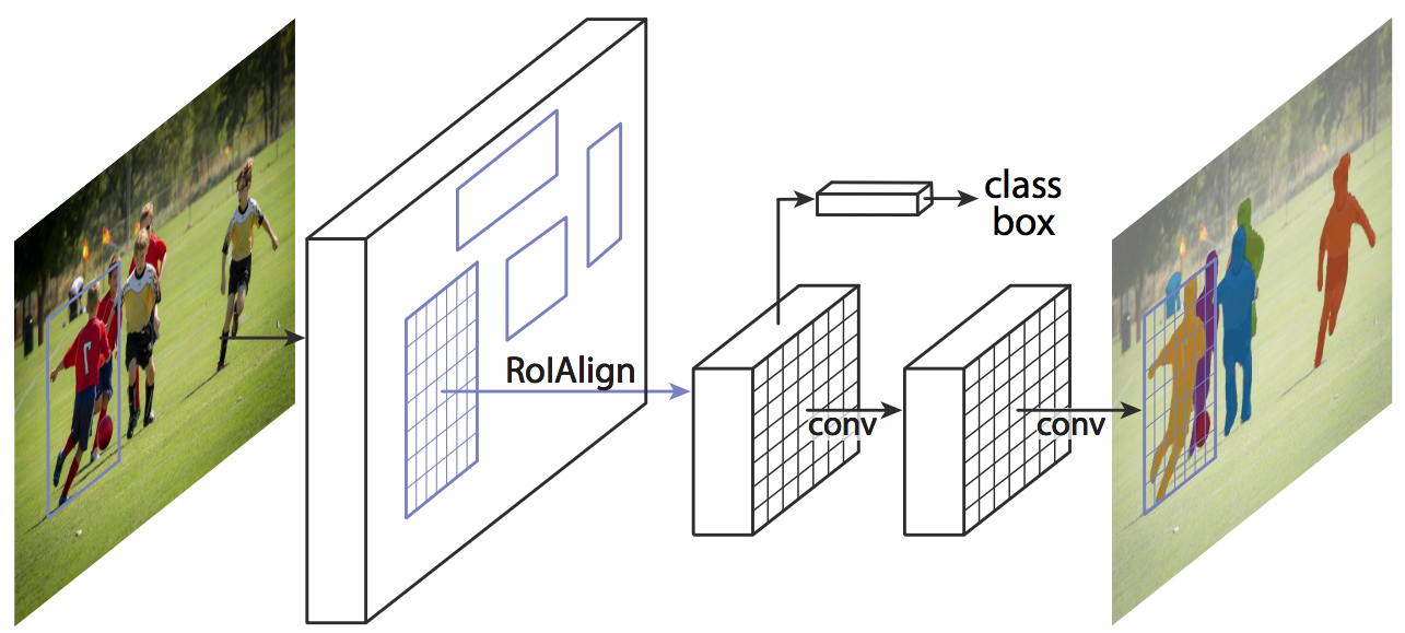
Mask R-CNN is an instance segmentation technique which locates each pixel of every object in the image instead of the bounding boxes. It has two stages: region proposals and then classifying the proposals and generating bounding boxes and masks. It does so by using an additional fully convolutional network on top of a CNN based feature map with input as feature map and gives matrix with 1 on all locations where the pixel belongs to the object and 0 elsewhere as the output.
Image segmentation
Partitioning a digital image into multiple segments (sets of pixels, also known as image objects). The goal of segmentation is to simplify and/or change the representation of an image into something that is more meaningful and easier to analyze. In particular, Mask R-CNN performs instance segmentation which means that different instances of the same type of object in the input image, for example, car, should be assigned to distinct labels. This project is mainly focused on car and trucks image segmentation.
2.1 Tensorflow
TensorFlow is an end-to-end open source platform for machine learning. TensorFlow is a rich system for managing all aspects of a machine learning system; however, this class focuses on using a particular TensorFlow API to develop and train machine learning models. See the TensorFlow documentation for complete details on the broader TensorFlow system.
TensorFlow APIs are arranged hierarchically, with the high-level APIs built on the low-level APIs. Machine learning researchers use the low-level APIs to create and explore new machine learning algorithms. In this class, you will use a high-level API named tf.keras to define and train machine learning models and to make predictions. tf.keras is the TensorFlow variant of the open-source Keras API.
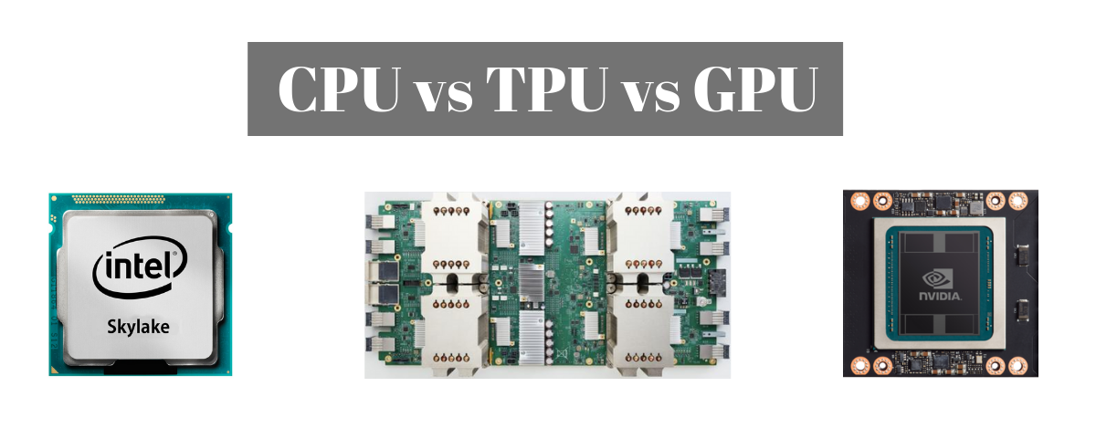
This setup of this project will allow you to run your Neural Network on TPU instead of traditional CPU. Tensor Processing Unit (TPU) is an AI accelerator application-specific integrated circuit (ASIC) developed by Google specifically for neural network machine learning, particularly using Google's own TensorFlow software. We will be using Google's TPU hosted runtime.
2.3 Google Colab set up
Mask R-CNN model addresses one of the most difficult computer vision challenges: image segmentation. Image segmentation is the task of detecting and distinguishing multiple objects within a single image.
Mask R-CNN model was trained on Cloud TPU to perform instance segmentation on a sample input image. The resulting predictions are overlayed on the sample image as boxes, instance masks, and labels. You need to open Google Colab and create a new notebook. So you can familiarize yourself with the platform.
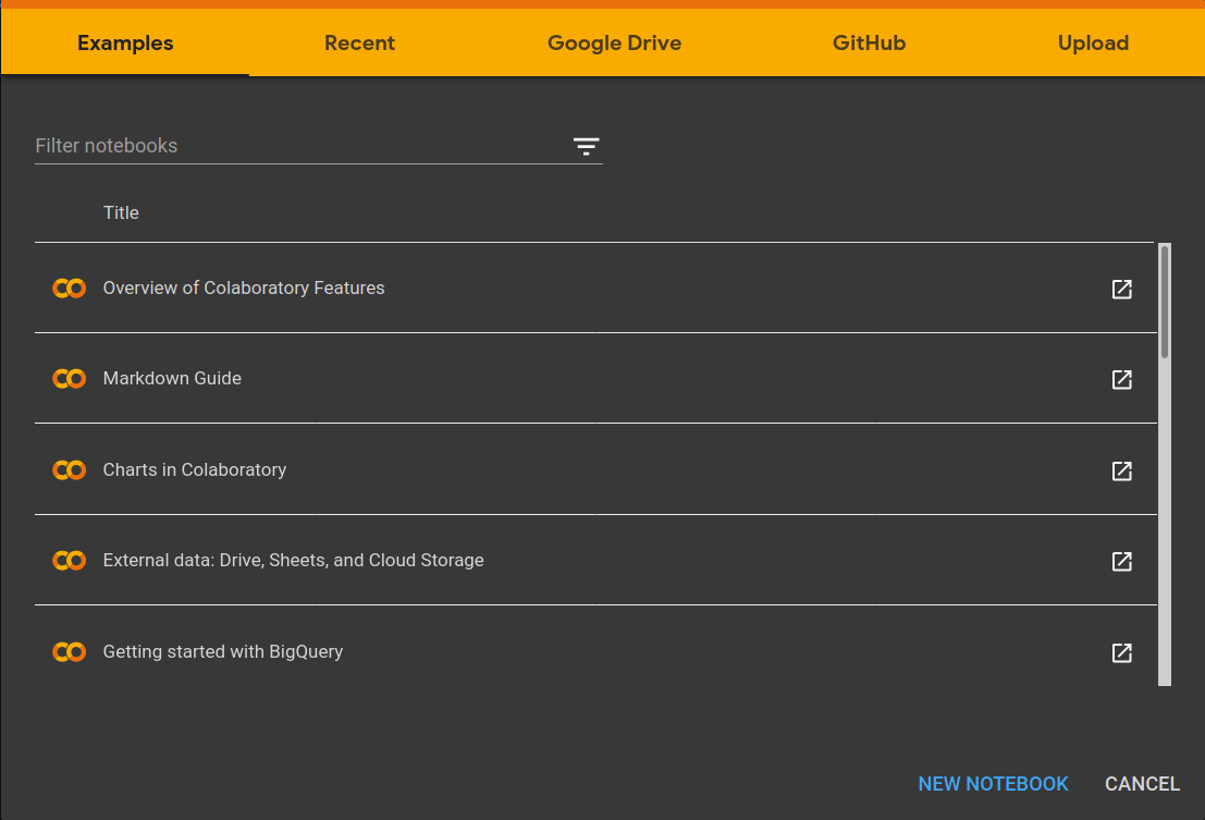
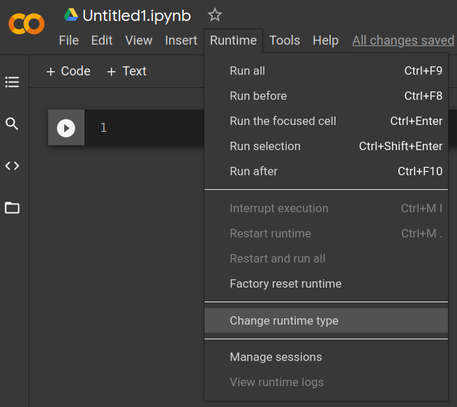
Once we created a new notebook, we have to change our runtime type. Click on Runtime option and select Change runtime type to TPU. Save the changes.
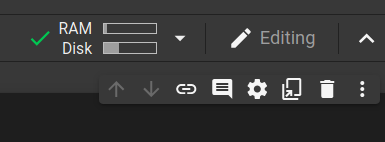
Now we click on connect at the top of the main bar. Once connected, we'll see RAM and Disk bars. From now on you can copy and paste the parts of the code in your own notebook.
2.4 Starting with the code
The full script can be found at the end of this chapter, but we are going to take a deep look to each fundamental part of the code to understand how the images are being processed
First, we have to download the source code of tensorflow and install requests module to make GET requests to Dropbox
!git clone https://github.com/tensorflow/tpu/
!pip install requests
You'll see an output like this:
Cloning into 'tpu'...
remote: Enumerating objects: 72, done.
remote: Counting objects: 100% (72/72), done.
remote: Compressing objects: 100% (55/55), done.
remote: Total 9870 (delta 29), reused 34 (delta 17), pack-reused 9798
Receiving objects: 100% (9870/9870), 24.31 MiB | 26.51 MiB/s, done.
Resolving deltas: 100% (7067/7067), done.
Requirement already satisfied: requests in /usr/local/lib/python3.6/dist-packages (2.23.0)
Requirement already satisfied: idna<3,>=2.5 in /usr/local/lib/python3.6/dist-packages (from requests) (2.10)
Requirement already satisfied: chardet<4,>=3.0.2 in /usr/local/lib/python3.6/dist-packages (from requests) (3.0.4)
Requirement already satisfied: certifi>=2017.4.17 in /usr/local/lib/python3.6/dist-packages (from requests) (2020.12.5)
Requirement already satisfied: urllib3!=1.25.0,!=1.25.1,<1.26,>=1.21.1 in /usr/local/lib/python3.6/dist-packages (from requests) (1.24.3)
TensorFlow 1.x selected.
Import necessary libraries and modules
#Import libraries
from IPython import display # display images
import pandas as pd # work with dataframes
from google.colab import files # work with files in colab
import requests # make get requests
from PIL import Image
from PIL import ImageFile
ImageFile.LOAD_TRUNCATED_IMAGES = True
import itertools # module to iterate easier over arrays
import numpy as np #use numpy arrays
%tensorflow_version 1.x
import tensorflow as tf # work with tensors
import sys
sys.path.insert(0, 'tpu/models/official')
sys.path.insert(0, 'tpu/models/official/mask_rcnn')
import coco_metric
from mask_rcnn.object_detection import visualization_utils
What is COCO? We are going to work with a pre-trained model, this means that we do not have to train our model with our data. This pre-trained model is called COCO. COCO is a large image dataset designed for object detection, segmentation, person keypoints detection, stuff segmentation, and caption generation. Here we create an index of object that our model will detect. Note that our main focus is on cars, trucks and buses, corresponding to labels 3, 8 and 6, respectively.
#Load COCO index mapping
ID_MAPPING = {
    1: 'person',
    2: 'bicycle',
    3: 'car',
    4: 'motorcycle',
    5: 'airplane',
    6: 'bus',
    7: 'train',
    8: 'truck',
    9: 'boat',
    10: 'traffic light',
    11: 'fire hydrant',
    13: 'stop sign',
    14: 'parking meter',
    15: 'bench',
    16: 'bird',
    17: 'cat',
    18: 'dog',
    19: 'horse',
    20: 'sheep',
    21: 'cow',
    22: 'elephant',
    23: 'bear',
    24: 'zebra',
    25: 'giraffe',
    27: 'backpack',
    28: 'umbrella',
    31: 'handbag',
    32: 'tie',
    33: 'suitcase',
    34: 'frisbee',
    35: 'skis',
    36: 'snowboard',
    37: 'sports ball',
    38: 'kite',
    39: 'baseball bat',
    40: 'baseball glove',
    41: 'skateboard',
    42: 'surfboard',
    43: 'tennis racket',
    44: 'bottle',
    46: 'wine glass',
    47: 'cup',
    48: 'fork',
    49: 'knife',
    50: 'spoon',
    51: 'bowl',
    52: 'banana',
    53: 'apple',
    54: 'sandwich',
    55: 'orange',
    56: 'broccoli',
    57: 'carrot',
    58: 'hot dog',
    59: 'pizza',
    60: 'donut',
    61: 'cake',
    62: 'chair',
    63: 'couch',
    64: 'potted plant',
    65: 'bed',
    67: 'dining table',
    70: 'toilet',
    72: 'tv',
    73: 'laptop',
    74: 'mouse',
    75: 'remote',
    76: 'keyboard',
    77: 'cell phone',
    78: 'microwave',
    79: 'oven',
    80: 'toaster',
    81: 'sink',
    82: 'refrigerator',
    84: 'book',
    85: 'clock',
    86: 'vase',
    87: 'scissors',
    88: 'teddy bear',
    89: 'hair drier',
    90: 'toothbrush',
}
category_index = {k: {'id': k, 'name': ID_MAPPING[k]} for k in ID_MAPPING}
2.5 Import Mask-RCNN pre-trained model
Once the category_index is defined, we create a TensorFlow session to run the inference.
The following lines of code will load a session that will help us to run our model. You can either connect to a TPU or a normal CPU backend. If you want to set up a local CPU runtime, you might need to follow the Setup instructions.
df_app = [] #aux variable
#Create a Tensorflow session to run the inference.
use_tpu = True
if use_tpu:
  import os
  import pprint

  assert 'COLAB_TPU_ADDR' in os.environ, 'Not connected to a TPU runtime;'
  TPU_ADDRESS = 'grpc://' + os.environ['COLAB_TPU_ADDR']
  print('TPU address is', TPU_ADDRESS)

  session = tf.Session(TPU_ADDRESS, graph=tf.Graph())
  print('TPU devices:')
  pprint.pprint(session.list_devices())
else:
  session = tf.Session(graph=tf.Graph())
Then, here we import our pre-trained model from public Google Clouds's bucket.
#Loading the coco pretrained seved model from the public GCS bucket
saved_model_dir = 'gs://cloud-tpu-checkpoints/mask-rcnn/1555659850'
_ = tf.saved_model.loader.load(session, ['serve'], saved_model_dir)
You will see an output like this:
TPU address is grpc://10.40.81.154:8470 TPU devices: [_DeviceAttributes(/job:tpu_worker/replica:0/task:0/device:CPU:0, CPU, -1, 16715985209963269316), _DeviceAttributes(/job:tpu_worker/replica:0/task:0/device:XLA_CPU:0, XLA_CPU, 17179869184, 883483035484795812), _DeviceAttributes(/job:tpu_worker/replica:0/task:0/device:TPU:0, TPU, 17179869184, 13302615515962944960), _DeviceAttributes(/job:tpu_worker/replica:0/task:0/device:TPU:1, TPU, 17179869184, 15404942215938030935), _DeviceAttributes(/job:tpu_worker/replica:0/task:0/device:TPU:2, TPU, 17179869184, 2479670436370698532), _DeviceAttributes(/job:tpu_worker/replica:0/task:0/device:TPU:3, TPU, 17179869184, 18187166108572051412), _DeviceAttributes(/job:tpu_worker/replica:0/task:0/device:TPU:4, TPU, 17179869184, 10695183106837905561), _DeviceAttributes(/job:tpu_worker/replica:0/task:0/device:TPU:5, TPU, 17179869184, 5187578072444121828), _DeviceAttributes(/job:tpu_worker/replica:0/task:0/device:TPU:6, TPU, 17179869184, 3135081301108399781), _DeviceAttributes(/job:tpu_worker/replica:0/task:0/device:TPU:7, TPU, 17179869184, 9092477821292355398), _DeviceAttributes(/job:tpu_worker/replica:0/task:0/device:TPU_SYSTEM:0, TPU_SYSTEM, 8589934592, 13869828514418346390)] WARNING:tensorflow:From:20: load (from tensorflow.python.saved_model.loader_impl) is deprecated and will be removed in a future version. Instructions for updating: This function will only be available through the v1 compatibility library as tf.compat.v1.saved_model.loader.load or tf.compat.v1.saved_model.load. There will be a new function for importing SavedModels in Tensorflow 2.0. INFO:tensorflow:Restoring parameters from gs://cloud-tpu-checkpoints/mask-rcnn/1555659850/variables/variables
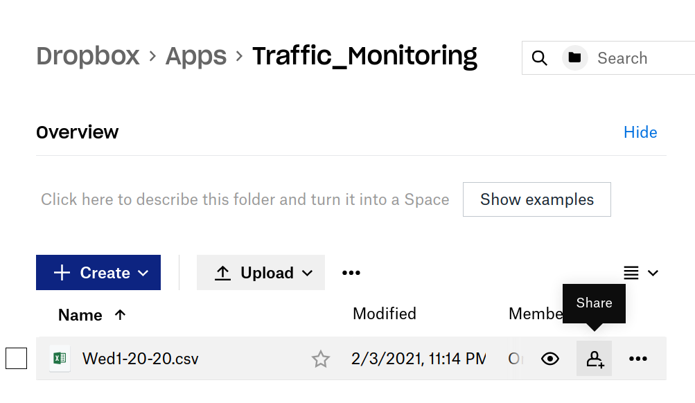
Now, copy and paste your link in to the read_csv() string parameter.
Note: You need to set the last 0 to 1 from the url in order to change the permission to read in a proper way the data

As mentioned in the previous chapter, we have renamed the headers of the columns in order to handle data easier
#Import previous generated csv from dropbox
  #set 1 at the end of the link
df = pd.read_csv("your_link_here/Wed1-20-20.csv?dl=1",
                 sep = ',',error_bad_lines=False)

#df.loc[:,'header_name'] returns all the vaules in the of the
#column according to the header name, we'll use 3 columns
images = df.loc[:,'Image']
cam_id = df.loc[:,'Cam_id']
timestamp_sg_time = df.loc[:,'Timestamp_sg_time']
url = df.loc[:,'Image']
2.6 For loop
This is the core of the script. We are going to use a for loop to process every image.
## Loading each image to apply the R-CNN
i = 1
# iterate over the number of pictures in the csv
for i in range(len(images)):
  # Make a GET request to the url of the image
  site = images[i]
  img_data = requests.get(site).content
  with open('image_name.jpg', 'wb') as handler:
      handler.write(img_data)

  image_path = 'image_name.jpg'

  with open(image_path, 'rb') as f:
    np_image_string = np.array([f.read()])
  #
  image = Image.open(image_path)
  width, height = image.size
  np_image = np.array(image.getdata()).reshape(height, width, 3).astype(np.uint8)

  # Comment the following line to hide the preview of the images
  display.display(display.Image(image_path, width=1024)) #Image preview
2.7 Perform instance segmentation and retrieve the predictions
Now let's run the inference and process the predictions from the model.
#Perform image segmentation and retrieve the predictions
  num_detections, detection_boxes, detection_classes, detection_scores,detection_masks, image_info = session.run(
      ['NumDetections:0', 'DetectionBoxes:0', 'DetectionClasses:0',
       'DetectionScores:0', 'DetectionMasks:0', 'ImageInfo:0'],
      feed_dict={'Placeholder:0': np_image_string})

  #Here are our variables that will contain all our useful data.
  num_detections = np.squeeze(num_detections.astype(np.int32), axis=(0,))
  detection_boxes = np.squeeze(detection_boxes * image_info[0, 2], axis=(0,))[0:num_detections]

  detection_scores = np.squeeze(detection_scores, axis=(0,))[0:num_detections]
  detection_classes = np.squeeze(detection_classes.astype(np.int32), axis=(0,))[0:num_detections]
  instance_masks = np.squeeze(detection_masks, axis=(0,))[0:num_detections]

  #coordinates of each detection box
  ymin, xmin, ymax, xmax = np.split(detection_boxes, 4, axis=-1)

  processed_boxes = np.concatenate([xmin, ymin, xmax - xmin, ymax - ymin], axis=-1)
  bounding_box_area = (xmax - xmin) * (ymax - ymin)
  segmentations = coco_metric.generate_segmentation_from_masks(instance_masks, processed_boxes,
                                                                              height, width)
  image_area = width * height
  proportion_bounding_box = (bounding_box_area / image_area)*100
It is worthy to mention you need to run all these lines of code inside the for loop (correct indentation). Once we have performed the image segmentation, let’s print the results with the following code:
#Visualze the detections results
  max_boxes_to_draw = 50
  min_score_thresh = 0.1

  # Our image iwth detections
  image_with_detections = visualization_utils.visualize_boxes_and_labels_on_image_array(
      np_image,
      detection_boxes,
      detection_classes,
      detection_scores,
      category_index,
      instance_masks=segmentations,
      use_normalized_coordinates=False,
      max_boxes_to_draw=max_boxes_to_draw,
      min_score_thresh=min_score_thresh)
  output_image_path = 'test_results.jpg'
  Image.fromarray(image_with_detections.astype(np.uint8)).save(output_image_path)

  # Comment the following line if you want to hide the output of each image.
  display.display(display.Image(output_image_path, width=1024)) #Processed image preview
Last but not least, we save all the predictions as a dataframe into a new csv file
#Create the dataframe with our lists
  df = pd.DataFrame(list(zip(itertools.repeat(i),itertools.repeat(cam_id[i]),
                             detection_classes, detection_scores,
                             itertools.repeat(timestamp_sg_time[i]),
                             itertools.repeat(url[i]))),
                columns =['Image_id', 'Cam_ID','Detection_Class', 'Detection_Score',
                                                        'Timestamp_sg_time','URL'])
  df_app.append(df)
  print(i,end=',')
#Download a simple dataframe with the detections classes and detection scores
df_simple = pd.concat(df_app)
#df_simple.set_index('Id', inplace=True)
print(df_simple)
df_simple.to_csv('Wed1-20-20.csv')
files.download('Wed1-20-20.csv')
Finally, a window will pop-up to save our file, here we select the path where we want to save our file.
You can find the full script of Mask RCNN in this Notebook. We have organized the full script only into two code cells to avoid a large number of request to Google Colab (they have limited free usage!). You may change adjust the url to your Dropbox App file and run it. Feel free to explore and play with the code.
You can find the full script of Huggingface Transformer in this Notebook.. You may change adjust the url to your Dropbox App file and run it. Feel free to explore and play with the code.
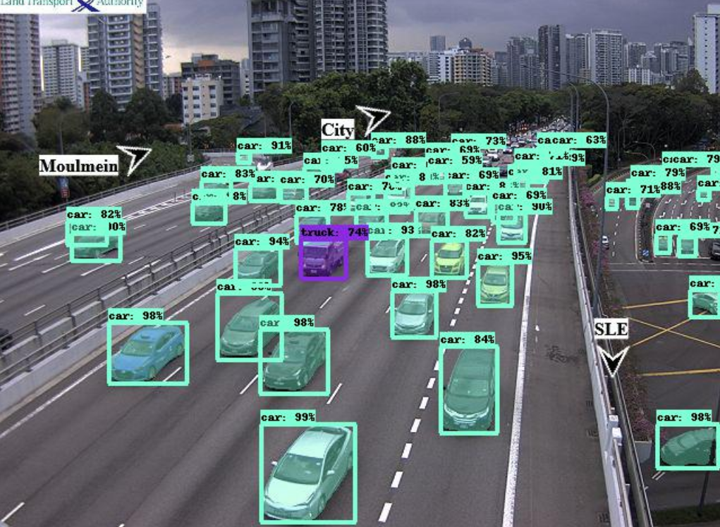
Here we have an example of a processed image, in this case the image #19 of our file that correspond to 2020-01-20 17:00:00 timestamp