Demographic Insights and Urban Features

In this section, we introduce code snippets that bring population data, building footprints, and elevation contours into the narrative.

Analyzing Population Counts

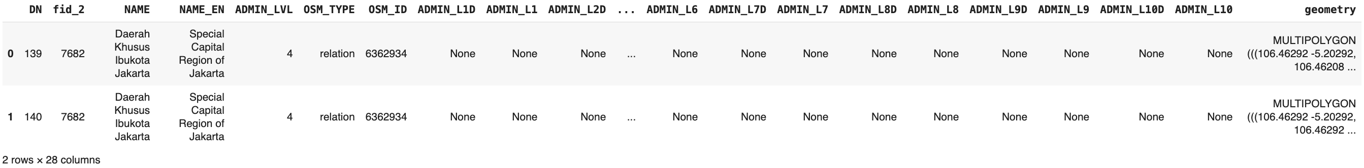
The following code snippet loads population data within the geographical boundary of Jakarta and provides insights into the demographic landscape:

The column 'DN' contains population counts.

    

POPULATION_GEOJSON_FILE = 'https://www.dropbox.com/scl/fi/cymqfopbx2df201f00sp8/
Population_Count_in_Jakarta_Boundary.gpkg?rlkey=ht2ks6o5qkqsm8wvgw9ljxvbe&dl=1'
# Read the GeoJSON file from the URL
population_gdf = gpd.read_file(POPULATION_GEOJSON_FILE)
    

print(f"Total columns: {population_gdf.shape[1]}")\
# Inspect the columns
population_gdf.head(2)



    Total columns: 28

    
print(f"Descriptive Statistics for Population counts:\n")
print(population_gdf['DN'].describe())
print(f"\nMissing Values : {population_gdf['DN'].isna().sum()}")
    

    
### output
Descriptive Statistics for Population counts:

count    41933.00000
mean       150.25226
std         35.63868
min         62.00000
25%        128.00000
50%        146.00000
75%        166.00000
max        239.00000
Name: DN, dtype: float64

Missing Values : 0
    

    
#### Plot
# Create a plot and specify the column for coloring
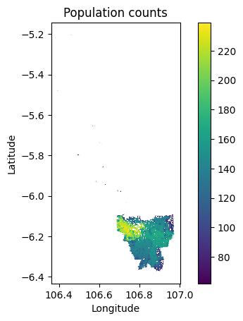
population_gdf.plot(column='DN', cmap='viridis', legend=True)

# Add title and labels
plt.title("Population counts")
plt.xlabel("Longitude")
plt.ylabel("Latitude")

# Show the plot
plt.show()
    

This code generates a map visualizing population counts within the specified geographical boundary, offering a spatial perspective on demographic distribution.

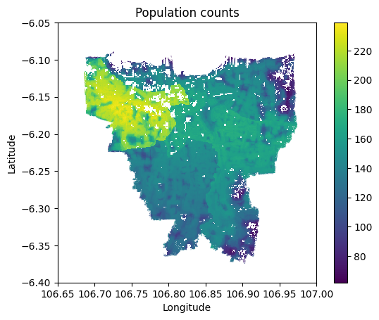
We can restrict the plot's x and y limits to focus on Jakarta City only

    
def plot_Jakarta_metric(sample_gdf,col_name, title, show_legend):
# Define the x and y limits
x_min, x_max = 106.65, 107.0
y_min, y_max = -6.4, -6.05

# Create a plot and specify the column for coloring
ax = sample_gdf.plot(column=col_name, legend=show_legend)

# Set x and y limits
ax.set_xlim(x_min, x_max)
ax.set_ylim(y_min, y_max)

# Add title and labels
plt.title(title)
plt.xlabel("Longitude")
plt.ylabel("Latitude")

# Show the plot
plt.show()

plot_Jakarta_metric(population_gdf,col_name='DN',title='Population counts',show_legend=True)
    

Exploring Building Footprints

Next, we bring building footprints into the spotlight, examining their spatial distribution and density:

    
import gdown

# Replace 'your_file_id_here' with the actual file ID
file_id = '1wuOhvtKege_gqql9-Xmnwd59wq2NAyWh'

# Construct the download link
file_url = 'https://drive.google.com/uc?id=' + file_id

# Specify the destination path where you want to save the file
output_path = '/content/building-polygon.gpkg'

# Download the file
gdown.download(file_url, output_path, quiet=False)

# Now, you can read the file using your preferred method
bldg_gdf = gpd.read_file(output_path)
print(bldg_gdf.columns)
print(bldg_gdf.shape)
bldg_gdf['item'] = 1
    
    
building_gdf =  bldg_gdf.copy()
building_gdf_projected = building_gdf.to_crs({'init': 'epsg:3857'})
building_gdf["area"] = building_gdf_projected['geometry'].area/ 10**6
building_gdf.head(2)
    
    

    
plot_Jakarta_metric(building_gdf,col_name='item',title='Building Counts',show_legend=False)
    

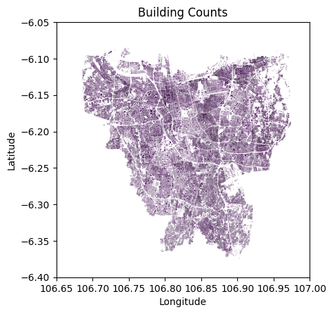
This code snippet loads building footprints, adds a dummy column, and calculates building areas. It sets the stage for understanding the spatial distribution and density of urban structures.

Elevation Contours

Lastly, elevation contours provide insights into the terrain of the city. The following function extracts elevation data for Jakarta:

    
import geopandas as gpd
import pandas as pd

def extract_elevation(city_folder_name):
    # Read the GPKG file into a GeoDataFrame
    dropbox_link = "https://www.dropbox.com/scl/fi/h9g2rjc49hbwc3ishf0o5/contour_lines.gpkg?rlkey=pdi83x7l6e3rrfvx8vjoghx98&dl=1"
    elevation_gdf = gpd.read_file(dropbox_link)

    print(elevation_gdf.head(2))

    # Specify the QML attribute(s) you want as a DataFrame
    qml_attribute = 'level'
    df = elevation_gdf[[qml_attribute]]

    # Perform operations on the DataFrame (e.g., df.head() to see the first few rows)
    #elevation_gdf(df.head())

    return elevation_gdf

elevation_gdf = extract_elevation('Jakarta_all_data')
print(elevation_gdf.shape)
elevation_gdf.level.unique(),elevation_gdf.cat.unique()
        
    
    
plot_Jakarta_metric(elevation_gdf,col_name='level',title='Elevation',show_legend=True)
    

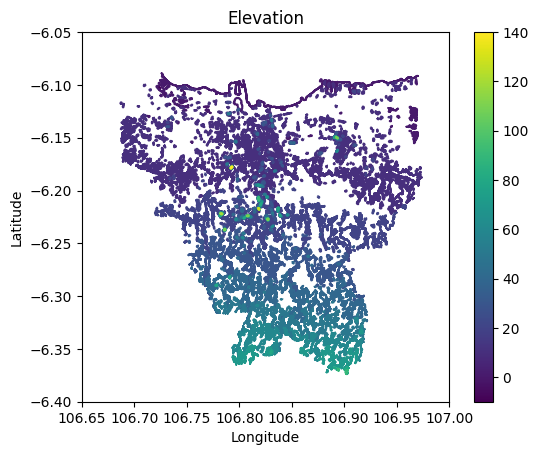
This function extracts elevation data and provides a glimpse into the topography of Jakarta.