Table of Contents

Extracting Pedestrian Networks: A Boundary-Based Approach

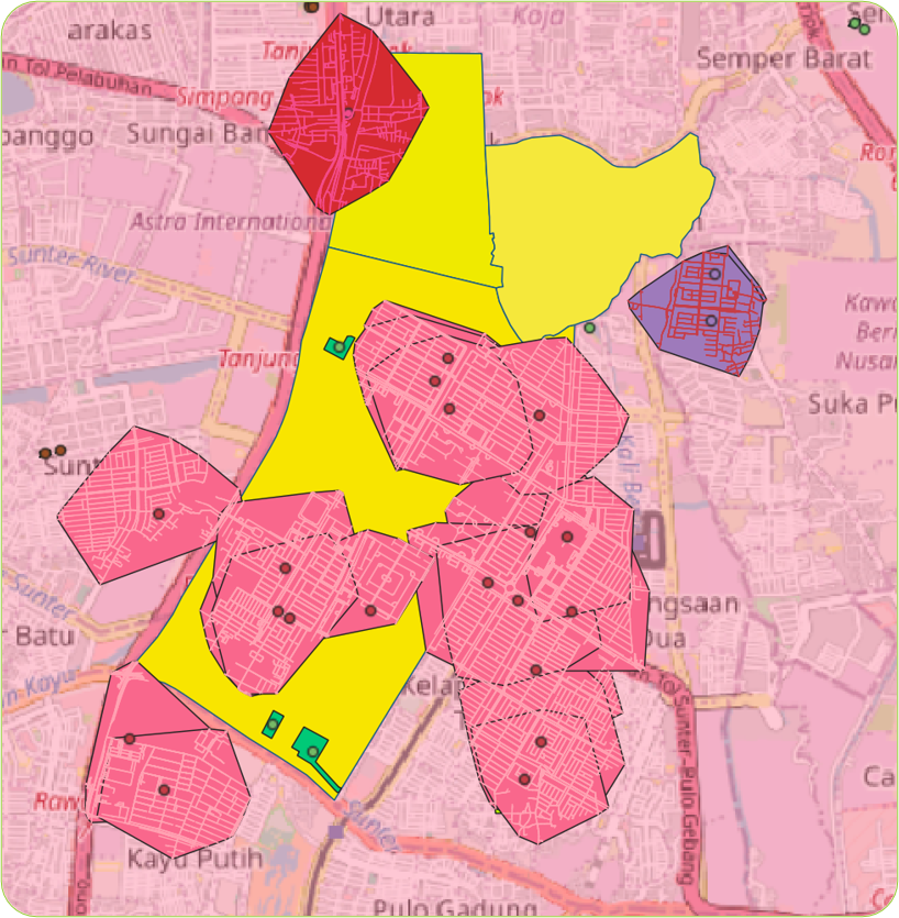
After setting up our Python environment with the necessary libraries, the next crucial step is to define the geographical boundaries of the city we want to analyze. This information is pivotal for extracting the pedestrian network within the specified area.

Unveiling the Pedestrian Network

Now that we have defined the geographical boundaries of our city using the boundary files, the next step is to extract the pedestrian network within this defined area. This is where the real exploration of walkability begins!

Quantifying Walkability: Measuring Network Length

One of the fundamental aspects of walkability is the physical length of pedestrian pathways within a city. In this section, we introduce a function that calculates and quantifies the total length of the pedestrian network in kilometers.

Quantifying Walkability: Assessing Network Density

In this section, we introduce a function that calculates both the total area of the defined boundary polygon and the network density.

Uncovering Intersections: Analyzing Intersection Density

In this section, we introduce a function that calculates both the total area of the defined boundary polygon and the network density.

Demographic Insights and Urban Features

In this section, we introduce code snippets that bring population data, building footprints, and elevation contours into the narrative.

Unveiling Walkability Metrics: Isochrone Analysis

The first step involves constructing an isochrone graph centered around a point of interest (POI) with latitude and longitude coordinates over our pedestrian network. The isochrone is created based on a specified walking distance (500 meters in this example) from the POI.

Unveiling Spatial Overlap: Walkability Metrics in Action

As we explore the intersection of walkability metrics within the isochrone and other geographical layers, our journey brings us to visualizing and calculating the density of the overlapping space.