Unveiling Spatial Overlap: Walkability Metrics in Action
As we explore the intersection of walkability metrics within the isochrone and other geographical layers, our journey brings us to visualizing and calculating the density of the overlapping space.
Plotting Spatial Overlap
The function plot_overlap allows us to visually inspect the spatial overlap between key walkability metrics, such as population density or building density or elevation, and the convex hull (isochrone)
# Define the x and y limits

def plot_overlap(geo_df_data,hull_gdf_sample, column_interested, insert_legend):
x_mins, x_maxs = 106.720, 106.732
y_mins, y_maxs = -6.158, -6.149

# Create a new figure
fig, ax = plt.subplots(figsize=(10, 10))
# Set x and y limits
ax.set_xlim(x_mins, x_maxs)
ax.set_ylim(y_mins, y_maxs)

# Plot the population counts on the axes
geo_df_data.plot(ax=ax, column=column_interested, cmap='viridis', legend=insert_legend)

# Plot the convex-hull (i.e., isochrone) on the same axes
hull_gdf_sample.plot(ax=ax, facecolor='none', edgecolor='black', lw=1)

# Add a legend to distinguish between the two datasets
ax.legend()

# Optionally, you can set the title and labels
ax.set_xlabel('Longitude')
ax.set_ylabel('Latitude')

# Display the plot
plt.show()
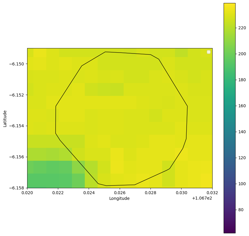
This function generates a plot showcasing the spatial overlap between the walkability metric (e.g., population density) or building density or elevation and the convex hull (isochrone).
To illuminate this intersection, we employ a series of functions that not only visualize the overlap but also quantify the density and distribution of these metrics within the defined walkable space.
We already know the total area of the isocrhone of interest, which is 0.6936 sq. km. We now need to observe how many people is living there in the 100m × 100 grid cells. We can first plot the population counts to have an idea of the desired result.
plot_overlap(population_gdf,hull_gdf, column_interested='DN',insert_legend=True)
Calculating Density in the Overlapping Area
To quantitatively assess the extent of overlap, we turn to the compute_density_overlap function. This function utilizes the geopandas.overlay method to calculate the spatial intersection between a walkability metric (e.g., population density) and the convex hull. The resulting overlap_gdf GeoDataFrame captures the specific geometries where these layers coincide, offering valuable insights into the geographical distribution of walkability metrics within the isochrone.
def compute_density_overlap(geo_df, hull_gdf_sample):
# Calculate the spatial overlap
overlap_gdf = gpd.overlay(geo_df, hull_gdf_sample, how='intersection')
# Count the number of rows in the overlapping GeoDataFrame
overlap_count = len(overlap_gdf)
print(f"Number of overlapping rows: {overlap_count}")
#print(overlap_gdf.DN)
# Plot
#ax = hull_gdf_sample.plot(facecolor='none', edgecolor='black', lw=1)
# Plot the overlapping geometries on the same plot
#overlap_gdf.plot(ax=ax, color='red', alpha=0.5)
# Save the plot
#plt.savefig('Overlap.png', column='DN', cmap='viridis', legend=True)
# Show the plot
#plt.show()
return overlap_gdf, overlap_count
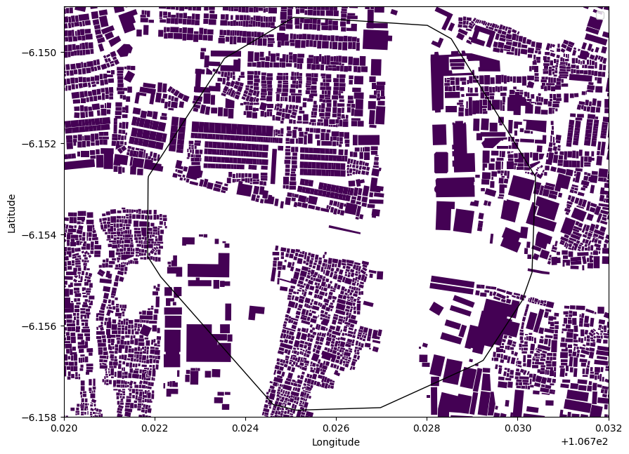
plot_overlap(building_gdf,hull_gdf, column_interested='item',insert_legend=False)
Insights into Walkability Metrics Overlap
After finding where walkability metrics overlap, the get_total_count function comes into play, shedding light on crucial details. It calculates the total count of the walkability metric within the overlapping space and provides density metrics.
overlap_gdf_elv, overlap_elv_count = compute_density_overlap(elevation_gdf, hull_gdf)

def get_total_count_(overlap_gdf,area_square_km, item_of_interest,  column_interested='DN'):
    total_population = overlap_gdf[column_interested].sum()
    area_square_km
    print(f"Total {item_of_interest}: {total_population}")
    print('Total area:', area_square_km)

    print(f"{item_of_interest} (per sq. km)): {total_population/area_square_km}")
get_total_count_(overlap_gdf_elv,area_square_km,  column_interested='level',item_of_interest='elevation')


Number of overlapping rows: 3
Total elevation: 30.0
Total area: 0.6936279316182797
elevation (per sq. km)): 43.250853422249044
For example, when we look at the total population within the overlapped region, and compute the population density (people per square kilometer), we gain a nuanced understanding of how walkability metrics are concentrated and distributed in the heart of the city. This calculation helps us gauge the density of essential factors, offering valuable insights into the urban landscape.