Unveiling Walkability Metrics: Isochrone Analysis

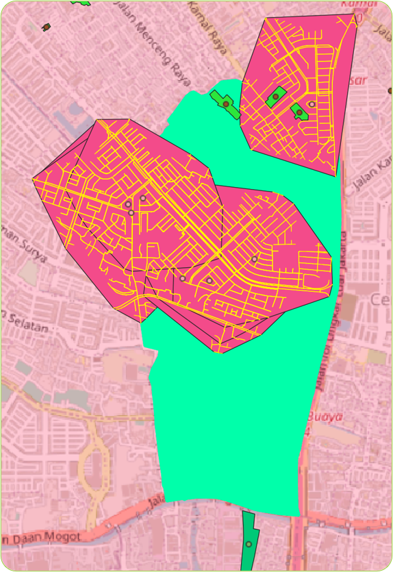
The first step involves constructing an isochrone graph centered around a point of interest (POI) with latitude and longitude coordinates over our pedestrian network. The isochrone is created based on a specified walking distance (500 meters in this example) from the POI:

    
from geopy.distance import geodesic

# Provide a point of interest with lat/lon coordinates
poi = (-6.153536, 106.726189)

# Compute the walking isochrone based on distance (500 meters in this example)
def compute_isochrone_for_poi(graph, poi, distance):
    isochrone = nx.MultiDiGraph()
    reachable_nodes = set()

    for node in graph.nodes(data=True):
        node_coords = (node[1]['y'], node[1]['x'])
        if geodesic(poi, node_coords).meters <= distance:
            reachable_nodes.add(node[0])
            # Add nodes to the isochrone
            isochrone.add_node(node[0], **node[1])

    for u, v, key, data in graph.edges(keys=True, data=True):
        if u in reachable_nodes and v in reachable_nodes:
            # Add edges to the isochrone
            isochrone.add_edge(u, v, key=key, **data)

    # Set the CRS for the isochrone (same as G2)
    isochrone.graph["crs"] = graph.graph["crs"]

    return isochrone

isochrone = compute_isochrone_for_poi(G2, poi, distance=500)
    

This function reads the pedestrian network data and constructs an isochrone graph, laying the foundation for subsequent walkability analyses.

Generating Convex Hull for Isochrone

We take a step further by defining the spatial extent of the isochrone through a convex hull analysis. This analysis creates a convex polygon encompassing the walkable area, offering a clearer visual representation.

The following code snippet defines a function, generate_convex_hull_for_isochrone(isochrone), which computes the convex hull for the coordinates of nodes within the isochrone:

    
from scipy.spatial import ConvexHull
from shapely.geometry import Polygon

def generate_convex_hull_for_iscochrone(isochrone):
    # Create a list to store the coordinates of nodes in the isochrone
    node_coords = []

    for node, data in isochrone.nodes(data=True):
        node_coords.append((data['x'], data['y']))

    # Compute the convex hull of the node coordinates
    hull = ConvexHull(node_coords)

    # Extract the convex hull vertices
    hull_vertices = [node_coords[i] for i in hull.vertices]

    # Create a Polygon from the convex hull vertices
    convex_hull_polygon = Polygon(hull_vertices)

    # Create a GeoDataFrame with the convex hull polygon
    hull_gdf = gpd.GeoDataFrame({'geometry': [convex_hull_polygon]}, crs=isochrone.graph["crs"])

    return hull_gdf

# Now you have a GeoDataFrame 'hull_gdf' containing the solid convex hull polygon
hull_gdf =  generate_convex_hull_for_iscochrone(isochrone)
    
    
def plot_hull_for_iscochrone(hull_gdf):
#### Plot
# Create a basic plot
hull_gdf.plot()
# Add title and labels
plt.title("Your isochrone")
plt.xlabel("Longitude")
plt.ylabel("Latitude")
# Show the plot
plt.show()
hull_gdf.columns

plot_hull_for_iscochrone(hull_gdf)
    

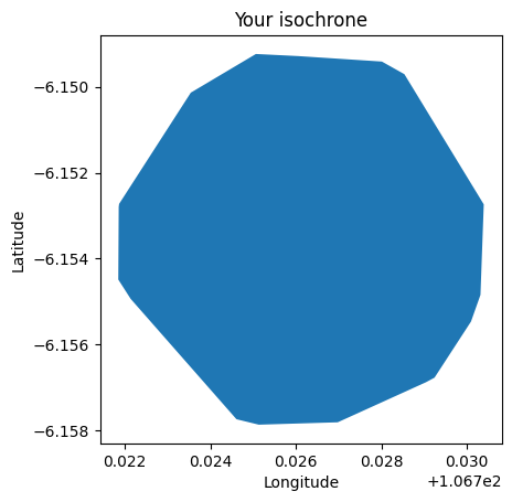
This function utilizes the scipy.spatial.ConvexHull algorithm to compute the convex hull of node coordinates within the isochrone. The resulting convex hull polygon is then encapsulated in a GeoDataFrame, hull_gdf, for further analysis.